Machine Learning at CMU
Overview
Four graduate projects from my first year at CMU, spanning reinforcement learning for robot manipulation, learning-augmented optimal control for drones, transformer-based generative models for image editing, and ML-based occupancy forecasting for smart buildings. Each project involved a full research cycle: problem formulation, implementation, evaluation, and analysis.
Robotic Learning — Franka Kitchen
Course: 16-831 Statistical Techniques in Robotics · Team: Sid Qian, Alexa Noto, Avi Dube · Code: https://github.com/AviDube/robot_learning_project
Overview
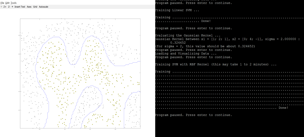
We studied how reward design and state representation affect reinforcement learning in the Franka Kitchen environment — a 9-DOF robot arm tasked with completing household manipulation goals (moving a kettle, opening cabinets, turning on burners). The environment uses sparse rewards by default, making it one of the harder benchmark settings in continuous-control RL.
We evaluated three learning algorithms (PPO, SAC, and model-based CEM) against a baseline, then proposed two modifications designed to improve training efficiency.
Baseline Algorithms
PPO was selected for its stability in continuous action spaces. Eight parallel environments ran via SubprocVecEnv, collecting diverse trajectories into a single shared policy update. It converged to a mean return of ~1.0 but struggled to consistently complete tasks under pure sparse reward.
SAC was paired with Hindsight Experience Replay (HER), which relabels failed trajectories with achieved goals to extract learning signal even from unsuccessful rollouts. SAC reached higher peak returns than PPO but exhibited significantly higher variance — HER sometimes reinforced partial behaviors that led to unstable Q-function updates.
Model-based RL (CEM) used a learned neural dynamics model combined with the Cross-Entropy Method for planning. CEM achieved faster initial improvement than both model-free methods by planning over predicted trajectories, but prediction errors accumulated over the planning horizon and limited long-term performance.
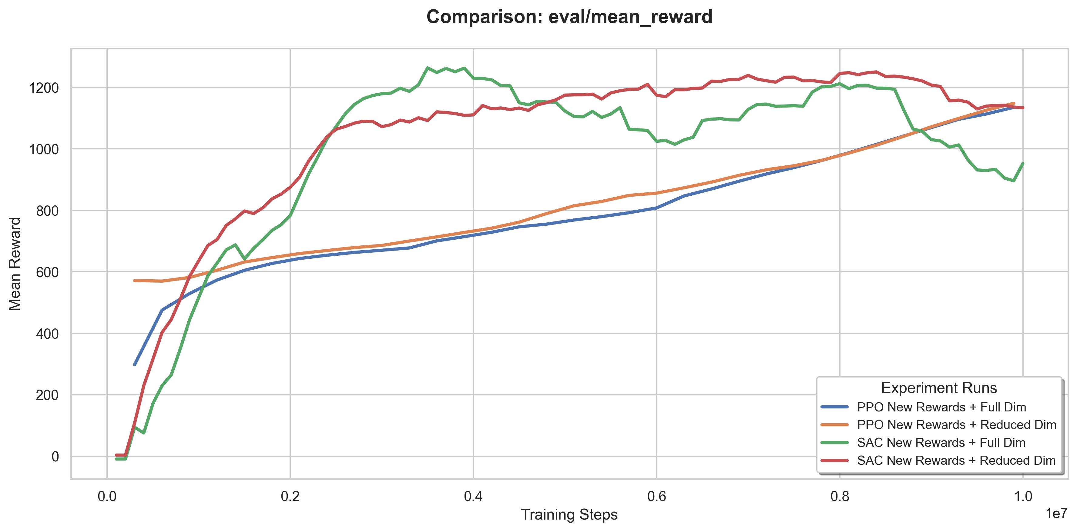
Training curves — PPO and SAC with dense reward + full/reduced state at 10M steps
Modification 1 — Dense Reward
The sparse reward only fires when a joint configuration lands within ε = 0.3 of the target. We augmented it with:
- Distance-to-goal: –‖s − g‖₂ providing continuous feedback proportional to proximity
- Element-wise sparse rewards: per-subtask completion signals
- Progress term: reward proportional to reduction in distance from the previous timestep
- Action regularization: penalty discouraging jerky control
- Time penalty: small per-step cost promoting efficiency
The dense reward produced smoother learning curves and significantly faster early improvement for both PPO and SAC. SAC benefited especially strongly — the dense signal addressed its core weakness of replay buffers dominated by unsuccessful transitions.
Modification 2 — Reduced State Representation
The default observation is a 59-dimensional vector including full proprioceptive state, object positions, velocities, and accelerations. We reduced this to only task-relevant features — end-effector pose and object positions — dropping velocities, accelerations, and redundant joint states.
This improved sample efficiency for PPO (faster early convergence, similar final performance) and stabilized SAC training. For model-based CEM, the reduced representation increased variance in the learned dynamics model, which degraded long-term performance.
PPO with Reduced Dim and New Rewards
SAC with Reduced Dim and New Rewards
Key Findings
Dense reward design had the larger impact on overall performance, enabling learning where sparse reward alone produced near-zero returns. Reduced state representation primarily affected efficiency and stability rather than final performance. PPO was the most stable across conditions; SAC reached higher peaks but required careful tuning; CEM was best at early-stage exploration but constrained by model accuracy.
MPC + Neural Lyapunov — Drone Control
Course: 16-745 Optimal Control and Reinforcement Learning · Team: Aniket Bhosale, Avi Dube · Code: github.com/AviDube/MPC-and-Lyapunov-for-drones
Overview
Quadrotor control is hard: the dynamics are nonlinear, coupled across translation and rotation, and sensitive to aerodynamic disturbances and sensor noise. Pure analytical models miss unmodeled effects; pure black-box models are hard to trust in safety-critical deployment. We built a hybrid pipeline combining first-principles physics with a learned residual dynamics model, embedded inside a nonlinear MPC controller, and then certified the controller’s stability using a learned neural Lyapunov function.
Simulation Environment
We built a high-fidelity MuJoCo simulation of a Crazyflie-style quadrotor with rigid-body dynamics, configurable wind disturbances, and domain randomization. The control loop runs at 50 Hz, mapping an optimized wrench command u = [T, τx, τy, τz] to four rotor thrusts via the quadrotor mixing matrix. The target task was hover stabilization at (0, 0, 1.2) m.
Residual Dynamics Learning
We first ran a baseline linear MPC (hover-linearized, solved with OSQP) to collect thousands of transition tuples (xₖ, uₖ, xₖ₊₁). The physics-based prediction fphys was computed via RK4 integration of the full rigid-body ODE including gravity, thrust, full rotation kinematics, and gyroscopic coupling.
The residual δθ = xₖ₊₁ − fphys(xₖ, uₖ) captures everything the analytical model misses — aerodynamic drag, rotor wake interactions, actuator dynamics. We parameterized δθ as a small MLP (3 hidden layers, 64 units, SiLU activations) trained with Huber loss and AdamW. SiLU was chosen because aerodynamic effects are smooth functions of state, and because SiLU(x) = x·σ(x) can be expressed symbolically in CasADi for automatic differentiation inside the MPC.
Nonlinear MPC with Hybrid Dynamics
Both fphys and δθ were expressed symbolically in CasADi, allowing IPOPT to differentiate through the full hybrid dynamics map automatically. The resulting NLP optimized over a 25-step (0.5 s) horizon with costs on state error, control effort, and input rate-of-change, plus a strong terminal penalty. Warm-starting from the previous solution kept the per-step solve within the 20 ms control budget.
The controller settled to the hover reference with no overshoot and near-zero steady-state attitude error. Benchmark sweeps confirmed tight z-axis tracking across a range of setpoints.
![]()
Benchmark sweeps of the NMPC controller across multiple reference trajectories.
Neural Lyapunov Certification
Because the closed-loop dynamics involve an NLP with learned components, a classical analytic stability proof is intractable. We used the generalized Lyapunov framework (Long et al., 2025) to train a data-driven certificate.
The candidate V(e) combines the MPC terminal cost Q_f (ensuring the certificate inherits the controller’s geometry) with a learned neural residual correction φθ₁ and a strict-positivity term β‖e‖². A second network σθ₂ allocates decrease requirements across a 30-step horizon, allowing delayed contraction — critical for underactuated systems that may temporarily grow position error while correcting attitude.
Both networks were trained by minimizing the hinge loss on the generalized decrease condition F(e) ≤ 0. On 30,000 held-out test rollouts, 99.80% of initial error states satisfied the decrease condition, providing strong empirical evidence of local stability across the certified hover region.
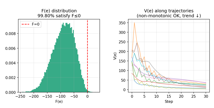
Generalized Lyapunov certificate diagnostics: training loss, horizon weight concentration $\sigma_i$, distribution of F(e) on the test set, and V(e) along sample trajectories.
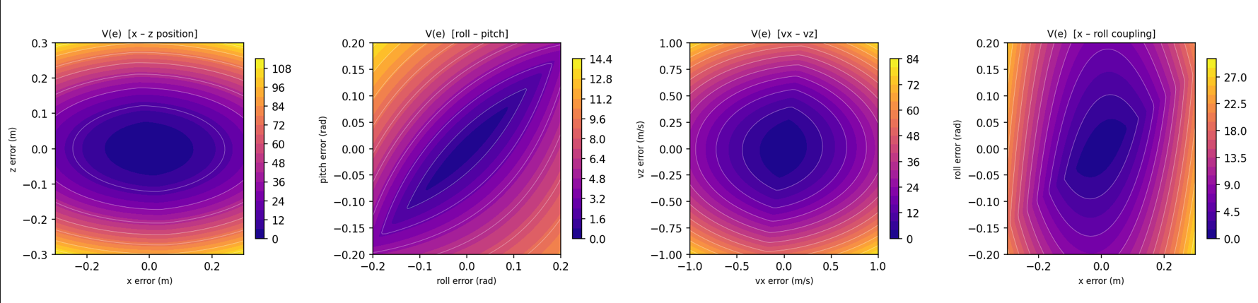
Two-dimensional slices of the learned Lyapunov function V(e) across position, attitude, velocity, and position–attitude coupling planes
Key Findings
The hybrid physics + residual model was accurate enough for the NMPC to plan trajectories the simulator faithfully executed, with no observable mismatch between predicted and realized closed-loop behavior. The neural Lyapunov certificate provides a practical post-hoc stability guarantee for a controller that cannot be certified analytically — a useful primitive for safety-critical deployment.
U-ViT Diffusion Backbone — Inversion-Free Image Editing
Course: 11-785 Introduction to Deep Learning · Team: Anirudh Mishra, Siddhi Apraj, Avi Dube, Yousha Mahamuni · Code: [github.com/Anirudh-Mishra/latent-style-shift]
Overview
Text-guided image editing usually requires expensive inversion of the input image into diffusion latent space. InfEdit (Couairon et al., 2023) avoids this using Denoising Diffusion Consistent Models (DDCM) and Unified Attention Control (UAC) — sharing attention maps between source and edit branches to preserve structure without inversion.
We investigated whether replacing InfEdit’s U-Net backbone with a U-ViT (U-shaped Vision Transformer) could improve structural preservation and edit fidelity by better capturing long-range dependencies.
Architecture
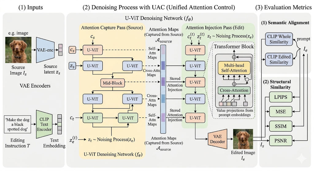
The pipeline encodes the source image Iₛ into latent space via a frozen Stable Diffusion VAE, and encodes the text instruction T via a frozen CLIP encoder. The U-ViT backbone processes the latent as non-overlapping patches through a symmetric encoder-decoder structure with long skip connections (mirroring U-Net’s multi-scale paths while operating on token sequences).
When source conditioning is enabled, the noisy target latent and clean source latent are channel-concatenated before patch embedding, doubling the input channels from 4 to 8. This gives every transformer layer explicit access to the source image structure.
UAC was adapted to the transformer setting via a two-pass mechanism: an attention capture pass records all cross-attention maps from the source branch, and an attention injection pass replaces the query-key alignment in the edit branch with stored source maps — enforcing spatial structure from the source while semantic content comes from the target prompt.
Architecture Diagram
Training Strategy
We tried four experimental paths:
- COCO fine-tuning — failed; COCO provides no source→edit pairs, so the model learned reconstruction rather than editing
- Knowledge distillation from a frozen LCM Dreamshaper U-Net teacher into a MAE-initialized U-ViT
- Edit-direction loss — explicit supervision matching the teacher’s predicted edit direction ε(z, edit) − ε(z, ∅), plus soft attention injection for structural consistency
- Option B — hybrid initialization combining MAE self-attention with bilinear-resized U-Net cross-attention, 10% CFG dropout, and same-latent probability = 1.0
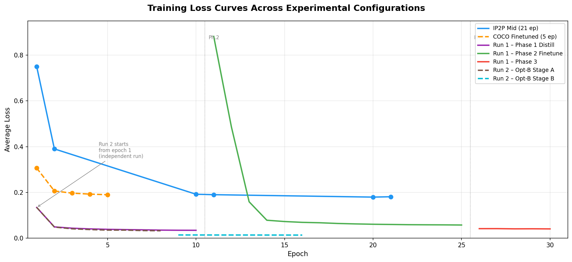
Training Loss Curves
Results
Our best configuration — mid-sized U-ViT trained on InstructPix2Pix for 21 epochs — was the only one that produced consistent, visible edits across the evaluation set.
| Metric | InfEdit (Baseline) | Our U-ViT (IP2P Mid) |
|---|---|---|
| CLIP Whole | 24.83 | 30.04 |
| CLIP Edited | 22.04 | 29.95 |
| LPIPS ×10³ | 56.10 | 217.40 |
| SSIM ×10² | 85.27 | 71.47 |
The U-ViT surpassed InfEdit on both CLIP metrics (+5.21 CLIP Whole, +7.91 CLIP Edited), showing it learned stronger instruction-following behavior. However, structural fidelity (LPIPS, SSIM) lagged behind — a consequence of UAC’s spatial grounding mismatch: UAC was designed for U-Net’s decoder layers where features have explicit spatial locality, whereas transformer attention is distributed globally across the token sequence.
Qualitative comparison — source images (bike, cat, woman), InfEdit outputs, U-ViT outputs
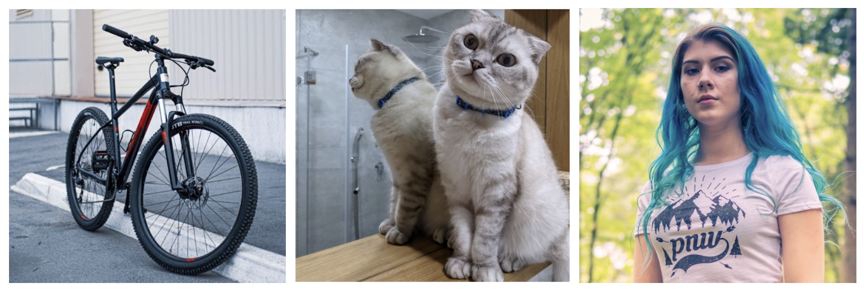
Original Images

Our Edits
Key Findings
Dataset choice was the most decisive factor: switching from COCO to InstructPix2Pix was what enabled edit-directed behavior, not architectural changes. Lower training loss did not guarantee better edits (Option B achieved the lowest loss but produced no visible edits). The pretraining gap between InfEdit’s U-Net (large-scale diffusion pretraining) and our U-ViT (MAE initialization) was the primary limiter of structural fidelity.
Occupancy Forecasting — CMU Smart Classrooms
Course: IoT and Smart Buildings · Team: Avi Dube, Dharun Muthaiah Nataraj, Stacy Godfreey-Igwe, Weronika Przedworska · Code: github.com/sg129646/CMU-ASB_OccupancyPrediction-Group
Overview
We built an end-to-end system to forecast classroom occupancy one day in advance across four rooms in a CMU academic building. The goal: give building managers actionable signals to reduce unnecessary HVAC, ventilation, and lighting in unoccupied spaces while maintaining comfort when rooms are in use.
Data Collection
Each room was instrumented with:
- An AMG8833 8×8 infrared thermal camera configured to detect heat blobs at doorways — counting people without capturing identifiable visual information
- An ESP32 Wi-Fi microcontroller pushing occupancy counts to a PostgreSQL database in real time
- 3D-printed sensor housing for stability
We supplemented the live sensor data with:
- Weather data (temperature, precipitation, wind speed) from the Open-Meteo API, updated hourly
- Classroom metadata from ScottyLabs Faculty Course Evaluations (FCE): meeting times, days, enrollment, FCE score, workload rating
All data was stored in a shared Supabase PostgreSQL instance. Training datasets were generated via SQL joins across room state, weather, holidays, and class schedule tables, aggregated at 30, 45, and 60-minute intervals.
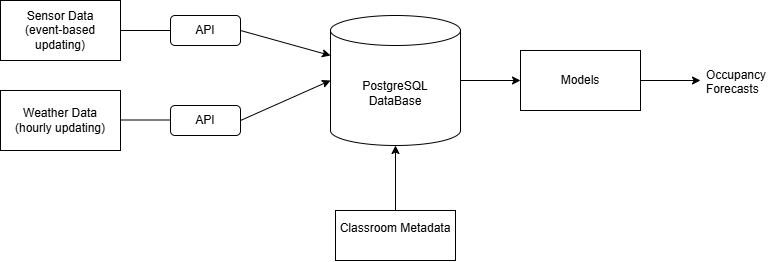
System architecture — sensor pipeline to PostgreSQL to ML models to occupancy forecast

Sensor setup — AMG8833 thermal camera mounted above doorway, connected to ESP32 microcontroller, housed in 3D-printed enclosure.
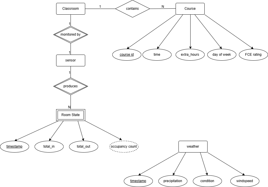
Entity-relationship diagram for the database schema
Models
We formulated occupancy prediction as a supervised multi-step time-series problem: given past occupancy and contextual features, predict the next 24 hours. Four models were evaluated:
Ridge Regression — linear mapping from flattened feature vectors (lags + temporal + schedule + weather) to multi-step outputs. Efficient and interpretable; performs best at coarser resolution (60-min) with long lag windows (72–96 hr).
XGBoost — gradient-boosted decision trees capturing non-linear feature interactions. Consistent MAE of ~1.75–1.85 across configurations.
Temporal Fusion Transformer (TFT) — LSTM encoder + multi-head attention sequence-to-sequence model. Accepts both past occupancy and known future covariates (schedule, time features). Best at 30-min resolution with 24-hr lag window; MAE as low as 0.36.
TimeLLM — GPT-2 based sequence forecasting model using only historical occupancy (no exogenous features). Despite receiving no schedule or weather context, it matched or exceeded TFT in several configurations — MAE as low as 0.36 at 30-min resolution.
Experiments
Configuration sweep: tested all combinations of 60/45/30-minute resolution × lag windows of 0/12/24/48/72/96 hours for all four models.
Feature ablation: removed one feature group at a time to measure impact:
| Feature Group | Impact |
|---|---|
| History (lag occupancy) | High — removing it degraded all models most severely |
| Temporal (hour, day of week) | High — especially critical for TFT |
| Schedule (in_session, FCE score) | High |
| Future covariates | Moderate |
| Capacity (static) | Negligible |
| Weather | Slightly negative — added noise in this dataset |
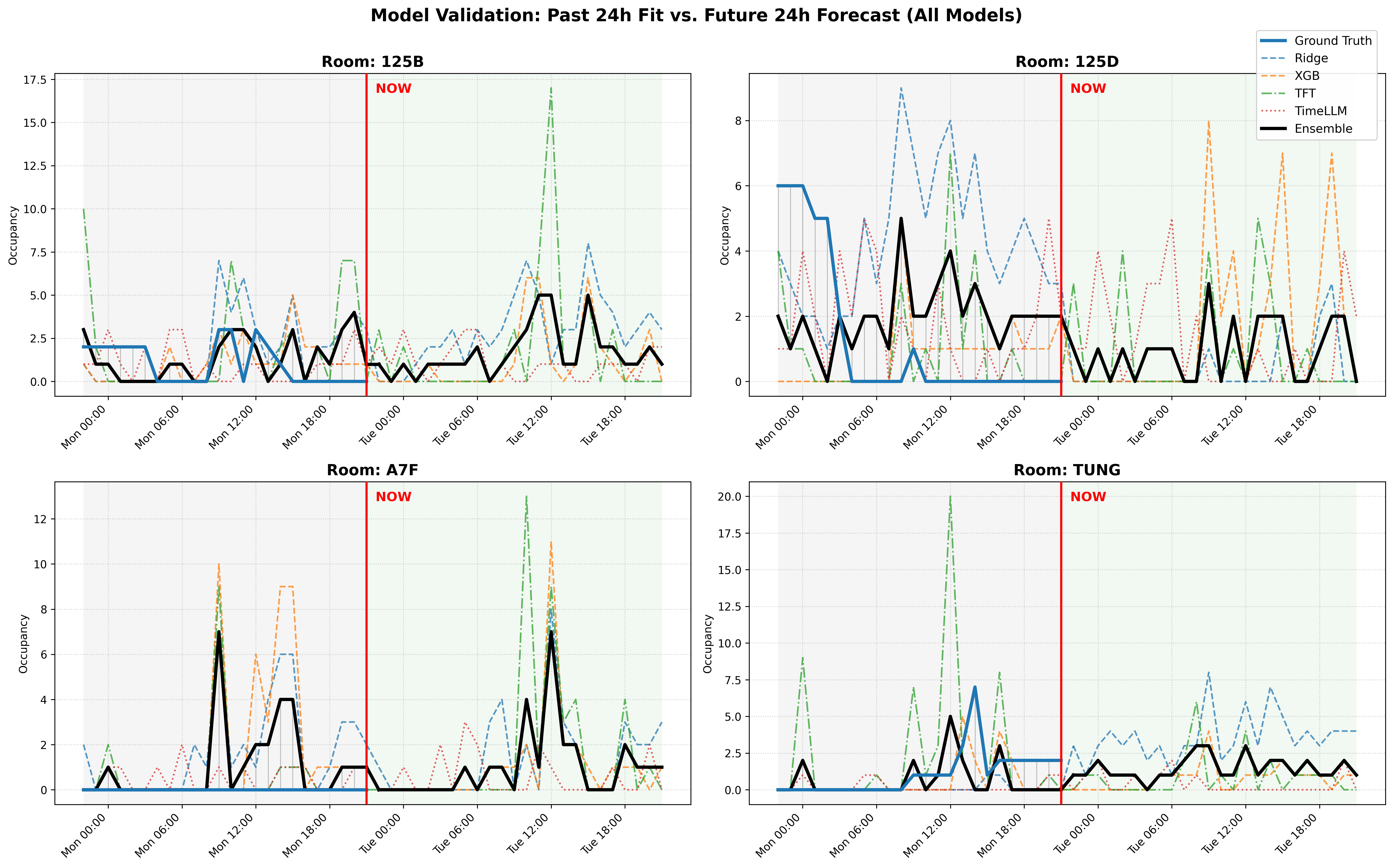
Model validation — past 24h fit vs. future 24h forecast across all four rooms
Key Findings
Sequence-based models (TFT, TimeLLM) consistently outperformed tabular methods by capturing temporal dependencies that flat feature vectors miss. Historical occupancy was by far the most important feature. Weather was a net negative in this dataset, suggesting indoor occupancy in structured academic buildings is largely decoupled from external conditions. TimeLLM’s strong performance without any exogenous features demonstrates that occupancy patterns contain strong intrinsic temporal structure.
Technologies
| Project | Key Tools |
|---|---|
| Franka Kitchen RL | Python · Stable-Baselines3 · Gymnasium · PPO · SAC · CEM |
| MPC + Lyapunov | Python · MuJoCo · CasADi · IPOPT · OSQP · PyTorch |
| U-ViT Image Editing | PyTorch · Stable Diffusion · CLIP · U-ViT · AdamW |
| Occupancy Forecasting | Python · PostgreSQL · XGBoost · PyTorch Forecasting · NeuralForecast |